GEOG 482
Final Project #3:
Remote Sensing Applications with LIDAR Systems for Enhanced Mountain Pine Beetle Kill Forest Surveys
Penn State University
Adam Knight

Figure 1: Mountain Pine Beetle Lifecycle. Retrieved on October 28th, 2014 from http://csfs.colostate.edu/images/graphics/barkbeetlefadergraphic.jpg
The mountain pine beetle has been a voracious eater of Colorado pine trees since 1996 (Mountain Pine Beetle (n.d.). Spanning from the Northern Rockies, all the down to the South Western United States, these beetles started their attack on the trees in Rocky Mountain National Park. They start by laying eggs underneath the pine tree bark. In the process of boring into the tree, they introduce a “blue stain fungus” into the sapwood which prevents the tree from expelling the beetles as a natural defense mechanism. This blue fungus also blocks the tree’s vital water and nutrient transport system. Eventually the whole tree becomes infested and dies off as a result. The colony attacks another neighboring tree and the cycle continues all over again over millions and millions of acres of forest lands to date (Mountain Pine Beetle CSU (n.d.). The current outbreak of Pine Beetle kill in the Colorado Rockies has been dramatic. Noticeable tracts of forest can be viewed for miles in every direction throughout most parts of Summit County Colorado. These dead trees pose a forest fire hazard and need to be clear cut as well as, monitoring for current attacks and projected outbreaks. A method for accurately tracking this beetle onslaught will be needed to quickly gather and analyze the data so scientists can developed a better strategy for protecting future generations of pine trees.
 |
|
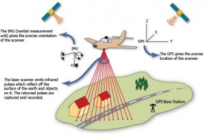
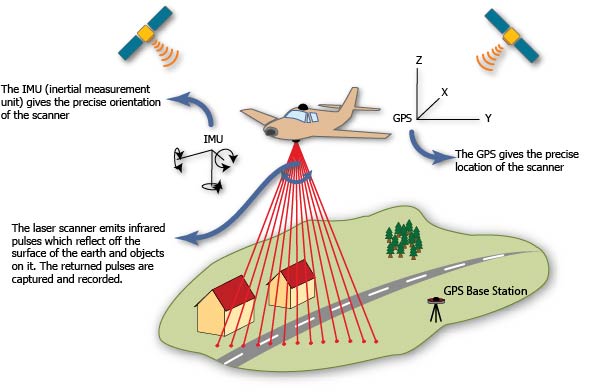
Figure 2: ALS
(Airborne Laser Scanning) coordinate the airplane’s speed, altitude, pitch, and
precise orientation to earth combined with satellite GPS location and ground-based
Base Stations Georeference LIDAR data in real-time during the scan. Retrieved
on October 28th, 2014 from http://gmv.cast.uark.edu/wp-content/uploads/2013/01/ALS_scematic-300x199.jpg
|
 |
|
Figure 3: LIDAR
returns can measure time, distance, and intensity to gather tree height and
canopy size. Retrieved October, 28th 2014 from http://www.imagingnotes.com/ee_assets/volume26/fernandez/figure2.jpg
|
Scientists have utilized a way to combine the high accuracy and point cloud data with the infrared spectral emission returns to monitor the vegetative decay of the trees through time. The spread of the Pine Beetles can be tracked utilizing point cloud data obtained from LIDAR and NDVI (Normalized Difference Vegetation Index) vegetation scans. Using a combined approach of cataloging tree data via LIDAR scans, hyperspectral images can be layered to give scientists the best possible approach to identifying green attack and red attack tree areas. NDVI can be shown as the equation: NDVI = (NIR — VIS)/(NIR + VIS). The measurements themselves are taken from a satellite named AVHRR (Advanced Very High Resolution Radiometer). The NDVI for the beetle kill can be seen in Figure 4 below. The gradual shading from light to dark shows the loss of tree foliage due to the spread of the Pine Beetles. A limitation of the NDVI is since is it satellite based, it can only resolve up to 1 km of landmass and the data takes about 2 weeks to process. Quicker scans be accomplished by mounting these near infrared scanners on planes with LIDAR systems for better resolutions and data turnaround processing times (Normalized Difference Vegetation Index (n.d.).
 |
|
Figure 4: The darker shaded
areas show higher tree mortality rates observed from Aerial Surveys. The darker
shaded areas are not indicative of total tree loss. Not all trees dead within
denser areas. Retrieved October 28th,
2014 from pdf: http://csfs.colostate.edu/pdfs/2013final-IDprogression-map.pdf
|
Figure 4: The darker shaded areas show higher tree mortality rates observed from Aerial Surveys. The darker shaded areas are not indicative of total tree loss. Not all trees dead within denser areas. Retrieved October 28th, 2014 from pdf: http://csfs.colostate.edu/pdfs/2013final-IDprogression-map.pdf
A team of scientists from the University of Idaho have taken this dual LIDAR and NDVI approach to a new level with added spectral carbon emissions taken from a Pine Beetle outbreak in the forests of Idaho. The team studied ACG (Aboveground Carbon) emissions from 2002 Pine Beetle outbreak which subsided in 2010. The study was called “Landscape-scale analysis of aboveground tree carbon stocks affected by mountain pine beetles in Idaho”. The team used four-band (blue, green, red, near-infrared), 0.2 digital aerial imagery for the study area. The results of the study were dramatic as seen in Figure 5:
“Tree mortality was positively spatially autocorrelated across the study area (p < 0.0001, Moran's I); i.e., areas of high mortality tended to be located adjacent to other areas of high mortality, suggesting clumped mortality (figure 1(a)). Generally, the study area contained four areas of severe mortality in the northwest corner, center, southwest corner, and southeast panhandle of the study area. Red trees, indicating more recent beetle activity, were generally located in the northern part of the study area. The western edge of the study area, where elevation is greatest, was less affected by bark beetles because forest composition is mixed at higher elevations, thereby including nonhost tree species.” (B C Bright, J A Hicke and A T Hudak (October 26, 2012).
 |
|
Figure 5: (44.3°N,
115.1°W) “Maps of per cent mortality cover (1 ha resolution) and per
cent aboveground carbon in killed trees (2.4 m map aggregated to 1 ha
resolution). Locations >2150 m elevation, within 91 m of roads,
and consisting of nonforested areas were excluded from analysis (white).” Retrieved
October 28th, 2014 from http://ej.iop.org/images/1748-9326/7/4/045702/Full/erl442339f1_online.jpg
|
Figure 5: (44.3°N, 115.1°W) “Maps of per cent mortality cover (1 ha resolution) and per cent aboveground carbon in killed trees (2.4 m map aggregated to 1 ha resolution). Locations >2150 m elevation, within 91 m of roads, and consisting of nonforested areas were excluded from analysis (white).” Retrieved October 28th, 2014 from http://ej.iop.org/images/1748-9326/7/4/045702/Full/erl442339f1_online.jpg
Once the team compared the tree mortality rates with AGC emissions, a spatial correlation was found which the team predicted before the study.
In summary, LIDAR systems can be used in many ways to accurately measure forest tree biomass structures such as height and canopy sizes quickly. Unfortunately, all the hardware for the laser scanners and image processors was initially costly about 5 years ago, but technology is becoming less expensive and thus the costs associated with LIDAR scanning are becoming much cheaper to produce. Now we are able to scale down the size and costs of the equipment into smaller packages such as UAV systems which mount the scanners and detectors on remote controlled helicopter drones (Breaking Through the Price Barrier for LIDAR Sensors (Sept, 2014). When combing the LIDAR systems with Hyperspectral imaging sensors, scientists are able to more viably analyze data from more than just tree heights and canopy sizes. They can monitor carbon emissions over time with dead beetle tree kill areas as well to obtain spatial correlations between dead trees and carbon emissions.
References:
B C Bright, J A Hicke and A T Hudak (October 26, 2012). Landscape-scale analysis of aboveground tree carbon stocks affected by mountain pine beetles in Idaho. Retrieved October 28th, 2014 from
Breaking Through the Price Barrier for LIDAR Sensors (Sept, 2014) In sUAS News. Retrieved on October 28th, 2014.
DiBiase, D. and others (2014). Nature of Geographic Information. The Pennsylvania State University. Retrieved October 28, 2014 from
Geospatial Modeling & Visualization (n.d.). Airborne Laser Scanning. Retrieved on October 28th, 2014 from
Mountain Pine Beetle CSU (n.d.). CSU Mountain Pine Beetle Research. Retrieved on October 28th, 2014 from
Mountain Pine Beetle (n.d.). In Wikipedia. Retrieved October 28th, 2014 from
Normalized Difference Vegetation Index (n.d.) In Wikipedia. Retrieved on October 28th, 2014 from http://en.wikipedia.org/wiki/Normalized_Difference_Vegetation_Index
USGS DEM (n.d.). In Wikipedia. Retrieved on October 28th, 2014 from